Following on a previous blog post on drawing fractals with LaTeX, today I am going to plot functions using LaTeX. As in the previous post, let’s start by preparing the LaTeX environment from scratch:

sudo apt-get install latex209-base latex209-bin latexmk texlive-full texlive-math-extra texlive-extra-utils texlive-generic-extra texlive-latex-extra

The pgfplots package for plotting functions and the standalone package for displaying the graph in a single document need to be installed manually as they are not currently present in the Ubuntu repositories:

# navigate to your local texmf folder (could also be ~/texmf or ~/.texmf)
cd ~/.texmf-var
# download the pgfplots package
wget http://sourceforge.net/projects/pgfplots/files/pgfplots/1.7/pgfplots_1.7.tds.zip/download
# unzip it in the texmf folder
unzip pgfplots_1.7.tds.zip -d .
# download the standalone package
wget  http://mirrors.ctan.org/install/macros/latex/contrib/standalone.tds.zip
# unzip it in the texmf folder
unzip standalone.tds.zip -d .
# update the texmf folder
texhash ~/.texmf-var
# remove the zip files
rm standalone.tds.zip pgfplots_1.7.tds.zip

To get started I am going to plot two simple functions which can be mathematically expressed as follows:

y = x * x
y = x / 2

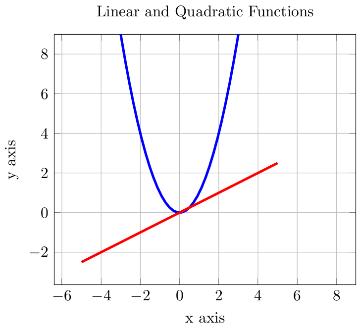
The first function is a linear function whose graph is a straight line. The second one is a quadratic function whose graph is a parabola. Here is the code to plot them with LaTeX:

\documentclass[border=2pt]{standalone}
\usepackage{pgfplots}
\pgfplotsset{compat=newest}
\begin{document}
\begin{tikzpicture}
    \begin{axis}[xmax=9,ymax=9,samples=50,grid=major,xlabel={x axis},ylabel={y axis},title={Linear and Quadratic Functions}]
    \addplot[blue, ultra thick](x,x*x);
    \addplot[red, ultra thick](x,x/2);
\end{axis}
\end{tikzpicture}
\end{document}

To compile the tex file into pdf from the command line you can use the latexmk utility previously installed and open the generated file with your preferred PDF editor (I use evince here).

latexmk -pdf plot_functions.tex
evince plot_functions.pdf &

The plotted functions look like this (and like this in PDF):

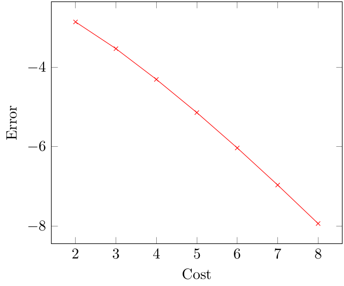
The next graph is obtained by joining a sequence of points whose coordinates on the x and y axis are clearly visible in the code (this example is adapted from the beautiful PGFPlots Gallery):

\documentclass[border=2pt]{standalone}
\usepackage{pgfplots}
\pgfplotsset{compat=newest}
\begin{document}

\begin{tikzpicture} 
    \begin{axis}[ xlabel=Cost, ylabel=Error] 
        \addplot[color=red,mark=x] coordinates {
        (2,-2.8559703) 
        (3,-3.5301677) 
        (4,-4.3050655) 
        (5,-5.1413136) 
        (6,-6.0322865) 
        (7,-6.9675052) 
        (8,-7.9377747)
    }; 
    \end{axis} 
\end{tikzpicture}

\end{document}

Again, I use latexmk to compile the code and evince to open the PDF.

latexmk -pdf plot_points.tex
evince plot_points.pdf &

The plotted function looks like this (and like this in PDF):

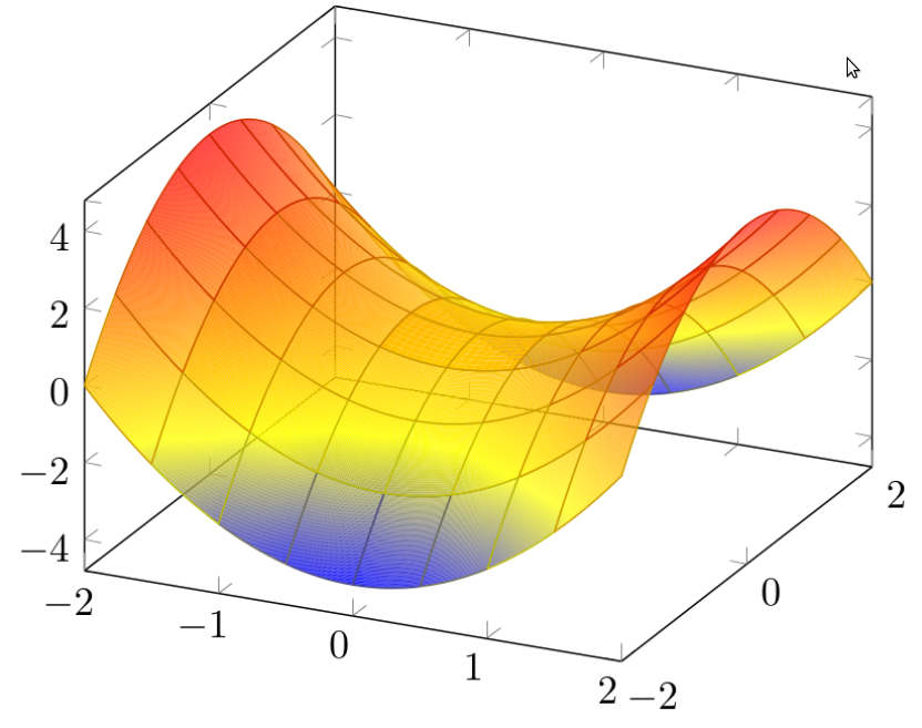
Finally, I’m going to draw a saddle surface. This is an example of hyperbolic geometry, a non-Eucledian geometry where the postulate of parallel lines doesn’t hold. Popular examples of hyperbolic geometry are the Pringles crisps and print works by the Dutch artist M. C. Escher. So here is the LaTeX code to generate a saddle surface:

\documentclass[border=2pt]{standalone}
\usepackage{pgfplots}
\pgfplotsset{compat=newest}

\pagestyle{empty}

\usepgfplotslibrary{patchplots}

\begin{document}
\begin{tikzpicture}
    \begin{axis}
    \addplot3[patch,patch refines=3,
		shader=faceted interp,
		patch type=biquadratic] 
    table[z expr=x^2-y^2]
    {
        x  y
        -2 -2
        2  -2
        2  2
        -2 2
        0  -2
        2  0
        0  2
        -2 0
        0  0
    };
    \end{axis}
\end{tikzpicture}
\end{document}

As usual, I compile it with latexmk and open it with evince.

latexmk -pdf saddle.tex
evince saddle.pdf &

And here is the beautiful saddle surface (and here is the associated PDF):

Sources:

Mihalis Tsoukalos, LaTeX: Make text beautiful, Linux Format 201, Summer 2015

http://pgfplots.sourceforge.net/gallery.html